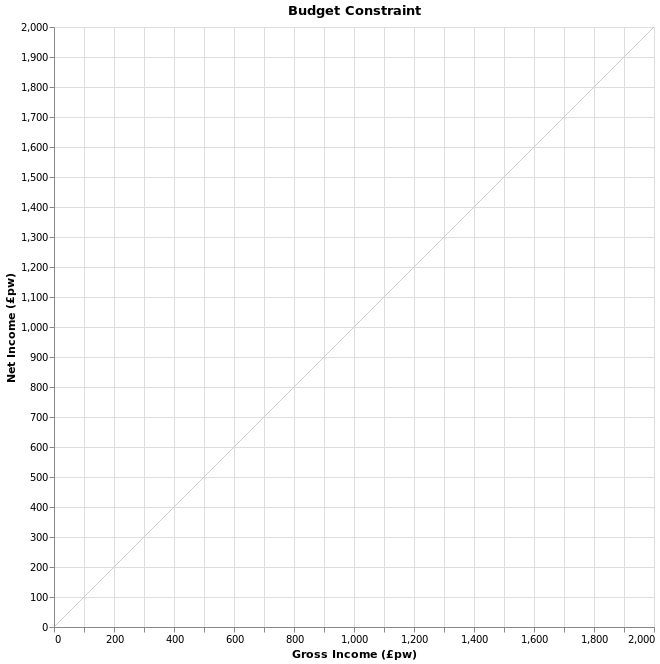

We’re going to start exploring our model by using it to generate a simple diagram: a budget constraint.
Above, to the left, we have some input fields you can use to sets up a simple income tax system. The first field is a tax allowance. This is the amount you can earn tax-free. Income above the tax allowance is taxable income. Underneath the allowance field, we have two fields for tax rates. We’ll call the first the basic rate and the second the higher rate. Below those is the higher rate threshold field. You pay at the basic rate till your taxable income exceeds the higher rate threshold, and any taxable income more than the threshold is taxed at the higher rate.
As an example, suppose your income was £40,000 per year, the allowance as £5,000, the basic rate 20%, the higher rate was 40% and the higher rate threshold £20,000. Then:
taxable income would be: * (40,000-5,000) = 35,000 *
tax at the basic rate would be:  * 20%×20,000 = 4,000 *
tax at the higher rate would be:  * (35,000-20,000)×40% = 6,000 *
so total tax due would be: * (4,000+6,000) = £10,000 *
Many tax systems have more than two rates (the Scottish system has five): I show two just to keep things simple. A complete description of the UK tax system would need a lot more than these four parameters, but I want to keep things as clear as possible for now. You can get a good feel for how a real world tax system works just with these four numbers.
A Note on periods A slightly confusing thing here is that the allowances and bands on the left are in £s per annum, whilst the graph is in £ per week. Taxes are normally expressed in annual amount, whilst benefits (and our FRS data) are normally expressed weekly or monthly. And from the next page on we’ll have taxes and benefits on the same page. I’ve tried to keep everything in its most natural units, but I appreciate this can be confusing at first.
On this page, the tax rates and allowances are initially set to zero - that may make it easier for you to see what the effects are of your choices of tax rates and allowances.
To the right of the inputs is our budget constraint graph. It shows for one person, or one family, the relationship between income before taxes (gross income) on the x- (horizontal) axis, and income after taxes have been taken off on the y- (vertical) axis. It’s often useful to think of the gross income as being pre-tax earnings.
The button at the bottom of the input fields sends your tax choices to the model, and the models does the needed suums and sends back a graph showing all the possible gross vs net income combinations for earnings from £0 to £2,000 per week1.
If there are no taxes (and no benefits - I’ll come to benefits in the next page), then if you earn £1, your net income will be £1, £100 gross gives you £100 net and so on. So the graph showing gross versus net income - the budget constraint - should simply be a 45% line up the middle of the chart. We invite you to check this by now by pressing the ‘run’ button with the default zero tax rates and allowance.
Now, I’d like you to experiment a little. Try setting the tax allowance and tax rates to some positive values just to get a feel for what happens.
In mainstream economics, people are assumed to make rational choices, choosing the best possible thing given their preferences and the constraints they face. An elaborate theory has been constructed about the nature of peoples preferences. But it turns out we don’t need much of this to get far in understanding choice - often all we need is to enumerate the constraints that they face, and the best choice is then often self-evident.
Economists draw budget constraints to help them understand all kinds of choices. In block XX week YY, you encountered one drawn between consumption now and consumption in the future, and you saw how that could help you understand savings decisions. Indeed, although not always drawn out, there are implicit budget constraints in practically everything in the course; for example between sugar and all other goods in the discussion of sugar taxes, or a ‘Government Budget Constraint’ in the cost-benefit-analysis week.
However, although it’s standard in the microsimulation field to call the graph we’re drawing here a budget constraint, it’s actually slightly different from the examples you normally find in textbooks. Crucially, I’m drawing this graph flipped round horizontally from the normal one.
When we analyse how direct taxes and benefits affect the economy, it’s natural to focus on the supply of labour - for a start, if a tax increase caused people to work less, it could backfire and cause revenues to fall. So he budget constraint that’s normally used to illustrate the choice of how much to work is set up in a slightly unintuitive way, so as to make it easy to analyse this aspect. The goods are consumption (usually on the y- axis) and leisure on the x- axis. So instead of studying the supply of labour directly, the analysis flips things round and studies the demand for leisure.
Every available hour not consumed as leisure spent working; that is exchanged for at consumption goods at some hourly wage.
In effect, the person’s wage is playing two roles here:
These two aspects of a wage - the ‘income effect and the ’substitution effect’ - work against each other, and are often thought to roughly cancel out, so increases or decreases in hourly wages might not make much difference to how much people want to work. Note that even if a tax increase has no effect on labour supply for this reason, it’s still effecting choices and hence welfare - a tax increase with no change in labour supply must mean that consumption of goods, and hence the welfare of the worker, is lower, and the price system is distorted.

Of course, this analysis needs to be modified in many ways - for example, many office workers might not get paid more if they stay late at work, or workers may be on fixed hours contracts and so unable to vary their hours, many people enjoy their work (at least up to some limit) and so on. Plus, of course, wages are not be the only source of income. Nonetheless, this the mainstream approach offers a simple but powerful analysis.
If you think about it, the key thing here is that consumers own a thing (their time) that is both a source of income and something that they want to consume directly (as leisure). Many economic problems have this characteristic. The two-period consumption versus saving example from block XX is an example. The choices of subsistence farmers between consuming their own crops or selling them at market is another.
We’ll use the budget constraint graph to introduce some important ideas: marginal tax rates, average tax rates, and replacement rates. Replacement rates make more sense when we can consider state benefits and taxes together, which we do in the next screen, so we’ll hold off on that one for now.
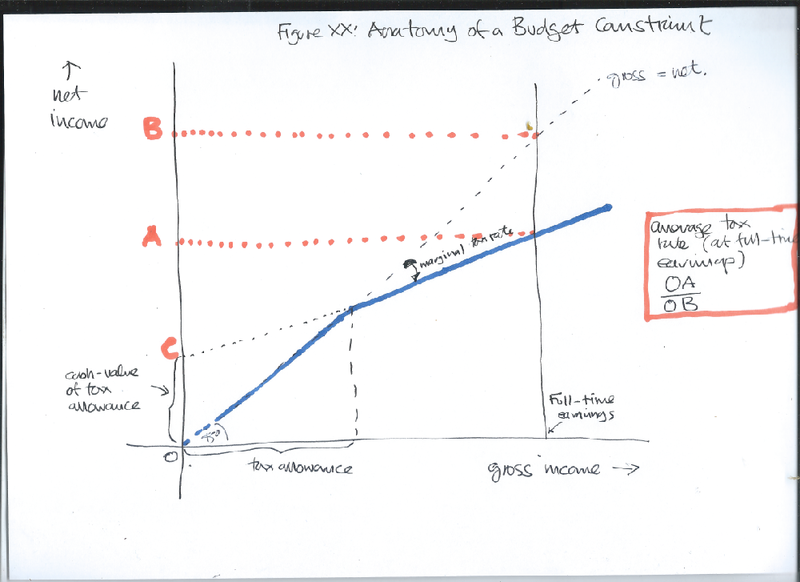
The Marginal tax rate (MTR) is the rate of tax on the next £1 that someone earns. We’ve seen in our discussion on fiscal neutrality that this is the key number for understanding how taxes distort the economy. In this case, it’s pretty easy to work out - since there is only one tax, with two tax rates and an allowance - the MTRs are 0, up to the tax allowance, then 20% up to the higher rate threshold, then 40% from then on. In the diagram, the MTR measures the extent to which the tax system flattens out the budget constraint compared to the 45° line - with a marginal rate of 0, you keep all of the next £ that you earn, with a MTR of 100% (which as we’ll see in a minute, is all too possible) you keep none of the next £1, so the budget constraint would be horizontal. If you hover your mouse over the points on the budget constraint, the program will display the MTR at that point.
The Average tax Rate is the proportion of total income you pay in tax. Some important choices are all-or-nothing rather than marginal, and for those, the average tax rate is more important than the marginal one. For example, back at the very start we saw a brief discussion of the fear that higher taxes in Scotland might encourage people to move to England. For this decision, people are choosing which side of the border they would to earn all of their income on, not just the next £12.
If the average tax rate rises with income, so a bigger proportion of income is taken in tax from rich people than poorer ones, the tax system is said to be progressive. Note that a progressive tax system doesn’t require marginal tax rates to be rising, so long as there is a tax allowance, since, with an allowance, the proportion of income that is taxable is higher for a rich person than a poorer one. We invite you to verify this by setting the basic and higher tax rates equal and examining the average tax rate at various points.
There’s one further measure that’s worth discussing here. Consider Edward, who earns £20,000 per anum. His tax allowance means that he has a taxable income of £10,000 (20,000-1000), and so pays tax of £2,000 (10,000×20%), with 20% also being his MTR. Ed would be in exactly the same position if he was taxed on all his income (so 20,000×20% or 4,000) and then given a tax-credit of £2,000, which is his tax allowance of £10,000 × his MTR of 20%. In other words his tax allowance has a cash value to him of £2,000. There’s much more to the tax and benefit system than the income tax we’re showing here, but no matter how convoluted the system gets, you can always summarise the entirety of someone’s position using just his MRT and this notional tax credit; this is a very useful trick when thinking about even the most complicated system3.
Figure XX below tries to summarise all these points in a stylised version of our budget constraint diagram.

Create a tax system a little like the UK one, with an allowance of £10,000, a basic rate of 20%, a higher rate of 40% and a higher rate threshold of £40,000 per annum.
Adam, Stuart, Mike Brewer, and Andrew Shephard. “Financial Work Incentives in Britain: Comparisons over Time and Between Family Types.” IFS, 2006. https://www.ifs.org.uk/wps/wp0620.pdf.
Callan, Tim, Michael Savage, and John R Walsh. “A Profile of Financial Incentives to Work in Ireland ESRI,” December 2015. https://www.esri.ie/publications/a-profile-of-financial-incentives-to-work-in-ireland.
Commission, Scottish Fiscal. “How We Forecast Behavioural Responses to Income Tax Policy March 2018.” Scottish Fiscal Commission, March 2018. http://www.fiscalcommission.scot/publications/occasional-papers/how-we-forecast-behavioural-responses-to-income-tax-policy-march-2018/.
Duncan, Alan, and Graham Stark. “A Recursive Algorithm to Generate Piecewise Linear Budget Contraints,” May 2000. https://doi.org/10.1920/wp.ifs.2000.0011.
the alogrithm needed to create a complete set see Duncan and Stark, “A Recursive Algorithm to Generate Piecewise Linear Budget Contraints.”.↩︎
see Commission, “How We Forecast Behavioural Responses to Income Tax Policy March 2018.” for a discussion.↩︎
see Callan, Savage, and Walsh, “A Profile of Financial Incentives to Work in Ireland ESRI.” for an application of these ideas to Ireland, and Adam, Brewer, and Shephard, “Financial Work Incentives in Britain.” for the UK.↩︎